Perspective
Deep Dive into VaR Calculation Methodologies
 Deep Dive into VaR Calculation Methodologies
Value at Risk (VaR) has become the industry standard metric for quantifying portfolio risk. Originally developed by JP Morgan in the 1990s, VaR answers a simple but crucial question: "What is the maximum loss I can expect over a given time period at a specified confidence level?" In building Scalata's risk engine, we implemented multiple VaR methodologies to give portfolio managers a comprehensive view of their risk exposures. This post explores these methodologies and the trade-offs between them.
 Understanding VaR
: The Basics
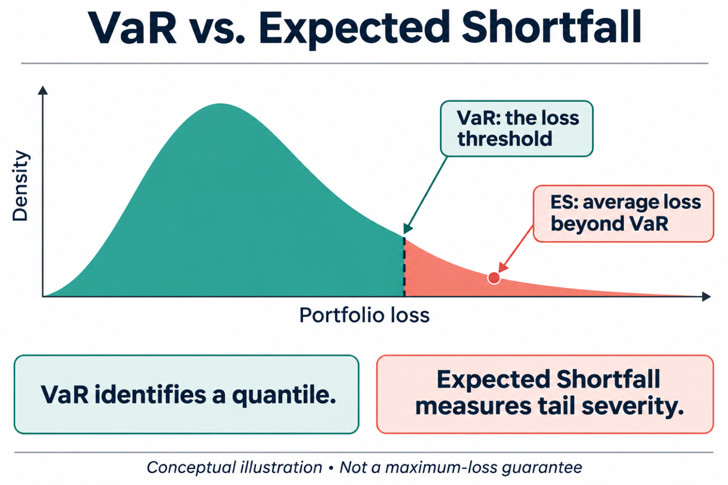
Before diving into methodologies, let's establish what VaR actually measures. A 1-day 95% VaR of $1 million means that, under normal market conditions, there is a 95% probability that the portfolio will not lose more than $1 million over the next trading day. Conversely, there is a 5% chance of losses exceeding this amount.
VaR is popular because it expresses risk as a single, intuitive number denominated in dollars (or the portfolio's base currency). This makes it easy to communicate to stakeholders, set risk limits, and compare risk across different portfolios or strategies.
However, VaR has important limitations. It says nothing about the magnitude of losses beyond the VaR threshold—the so-called "tail risk." A portfolio with a $1 million VaR might have expected tail losses of $1.5 million or $5 million; VaR alone doesn't distinguish between these cases. This is why we also calculate Expected Shortfall (ES), also known as Conditional VaR, which measures the average loss in the tail beyond the VaR threshold.
Historical Simulation VaR
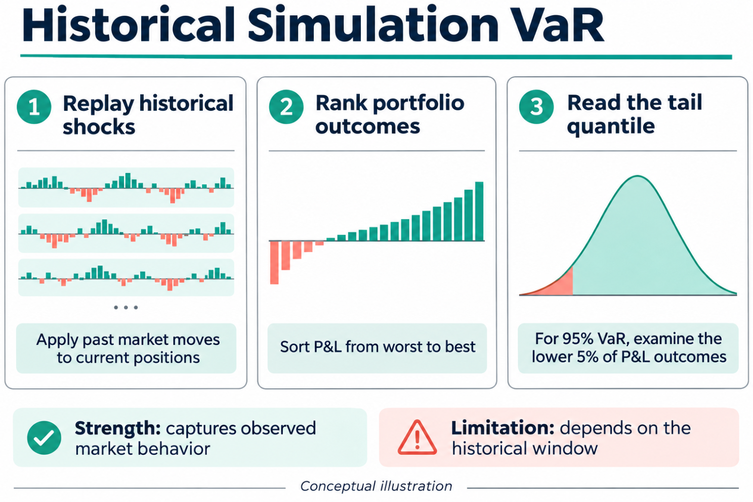
The most intuitive VaR methodology is historical simulation. The approach is straightforward: apply historical market returns to the current portfolio and observe the distribution of simulated P&L outcomes.
 Historical Simulation VaR
For example, if we're calculating 1-day VaR using 500 days of historical data, we calculate what the portfolio's return would have been on each of those 500 days given current positions. We then sort these 500 simulated returns from worst to best. For 95% VaR, we take the 25th worst return (the 5th percentile) as our VaR estimate.
Advantages: Historical simulation makes no assumptions about the distribution of returns. It naturally captures fat tails, skewness, and complex correlation structures that existed in the historical data. It's also easy to explain to non-technical stakeholders.
Disadvantages: Historical simulation assumes that the future will resemble the past. If the historical window doesn't include a market stress event, the VaR estimate may understate tail risk. Conversely, if a one-time event is included in the window, it may overstate ongoing risk. The methodology also requires substantial historical data, which may not be available for newer instruments.
In Scalata, we implement historical simulation with configurable lookback windows (typically 250-500 trading days) and offer options for exponentially weighted historical simulation, which gives more weight to recent observations.
Parametric (Variance-Covariance) VaR
 Parametric VaR
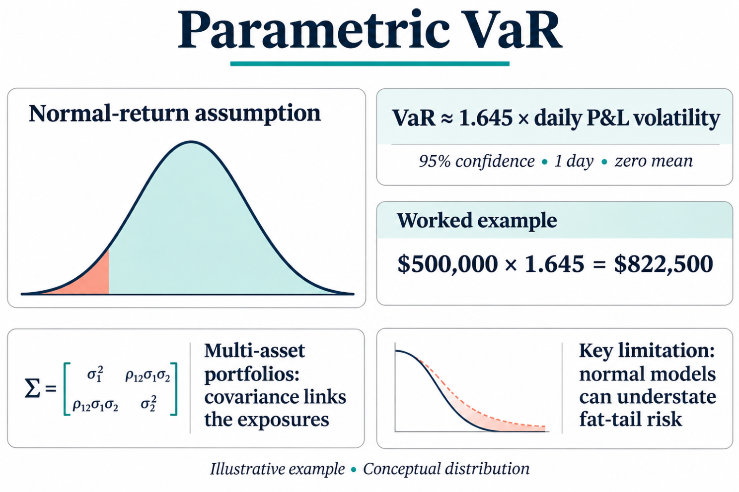
 takes a different approach, assuming that portfolio returns follow a known distribution—typically the normal (Gaussian) distribution. Under this assumption, VaR can be calculated analytically using the portfolio's expected return, volatility, and the appropriate z-score for the confidence level.
For a 95% confidence level, the z-score is approximately 1.645. If a portfolio has daily volatility of $500,000, the 1-day 95% parametric VaR would be approximately $822,500 (1.645 × $500,000).
For multi-asset portfolios, parametric VaR requires estimating the covariance matrix of asset returns. The portfolio variance is then calculated as the quadratic form of position weights and the covariance matrix.
Advantages: Parametric VaR is computationally efficient and can be calculated almost instantaneously, even for large portfolios. It provides a clear analytical framework that facilitates sensitivity analysis and marginal risk calculations.
Disadvantages: The normality assumption is often violated in practice. Financial returns typically exhibit fat tails (more extreme events than predicted by the normal distribution) and negative skewness (larger downside moves than upside). Parametric VaR tends to underestimate tail risk during market stress.
Scalata's parametric VaR implementation uses robust covariance estimation techniques, including shrinkage estimators and exponentially weighted moving averages, to improve the stability and accuracy of covariance estimates.
Monte Carlo Simulation VaR
 Monte Carlo Simulation VaR
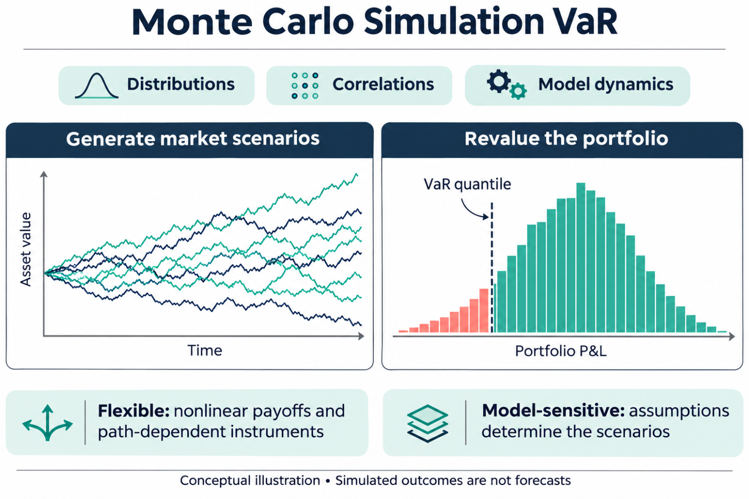
Monte Carlo simulation offers the most flexible approach to VaR calculation. Rather than relying solely on historical data or analytical formulas, Monte Carlo generates thousands of simulated market scenarios based on specified statistical models.
The process involves: (1) specifying a model for asset returns, including distributions, correlations, and any dynamic features like volatility clustering; (2) generating thousands of random scenarios from this model; (3) calculating portfolio P&L under each scenario; and (4) determining VaR from the resulting P&L distribution.
Advantages: Monte Carlo can accommodate any distributional assumptions, including fat tails, skewness, and complex dependency structures like copulas. It can also model path-dependent instruments like options and structured products, where the payoff depends on the entire price path, not just the final price.
Disadvantages: Monte Carlo is computationally intensive, requiring thousands or millions of simulations for accurate results. The quality of results depends heavily on the quality of the underlying model—garbage in, garbage out.
In Scalata, we implement Monte Carlo VaR with configurable simulation counts (typically 10,000-100,000), support for multiple distributional assumptions (normal, Student-t, and custom), and variance reduction techniques to improve computational efficiency.
Choosing the Right Methodology
Each VaR methodology has its place, and sophisticated risk managers use multiple approaches in combination. Historical simulation provides a reality check grounded in actual market experience. Parametric VaR offers computational efficiency and analytical tractability. Monte Carlo provides flexibility for complex portfolios and stress testing.
Scalata presents all three methodologies side-by-side, allowing users to compare results and understand where they diverge. When methodologies disagree significantly, it often signals that the portfolio has characteristics—like option exposures or concentrated positions—that warrant closer examination.
Beyond VaR: Component and Marginal Risk
Understanding total portfolio VaR is just the starting point. Scalata also decomposes VaR into component contributions, showing how much each position contributes to total portfolio risk. This enables portfolio managers to identify risk concentrations and evaluate the risk-adjusted attractiveness of individual positions.
Marginal VaR shows how portfolio risk would change with small changes in position sizes, guiding decisions about position sizing and portfolio construction. These tools transform VaR from a passive reporting metric into an active portfolio management tool.